Overview
fireR provides convenient access to USGS fire datasets and EPA/CEC ecoregion boundaries:
-
get_mtbs()/read_mtbs()for MTBS (Monitoring Trends in Burn Severity) wildfire perimeter data -
get_sefire()for SE FireMap data products (Burn Severity mosaics 2000–2022; Fire History, Burned Area Polygons, and Burned Area Rasters 1994–2024) -
get_nifc()/read_nifc()for NIFC (National Interagency Fire Center) wildfire perimeters -
get_fod()/read_fod()for the USFS Fire Occurrence Database (FPA-FOD, 1992–2020) -
get_wui()for the USFS Wildland-Urban Interface (WUI) dataset -
get_nal1eco(),get_nal2eco(),get_nal3eco()for CEC North America ecoregion boundaries -
get_usl3eco(),get_usl4eco()for US EPA ecoregion boundaries
A quick look
Most fireR functions pull large archives straight from the source, so
the examples below are not run when this site is built. The maps in this
section, however, are produced live from a single, modest download — the
CEC North America Level 1 ecoregion boundaries — to show what the
returned spatial objects look like with both base R plot()
and ggplot2.
library(ggplot2)

# A single, reliably-hosted download (~tens of MB)
na_l1 <- get_nal1eco(verbose = FALSE)
Base R plot() of an sf object, coloured by
ecoregion name:
plot(na_l1["NA_L1NAME"], main = "North America Level 1 Ecoregions", border = NA)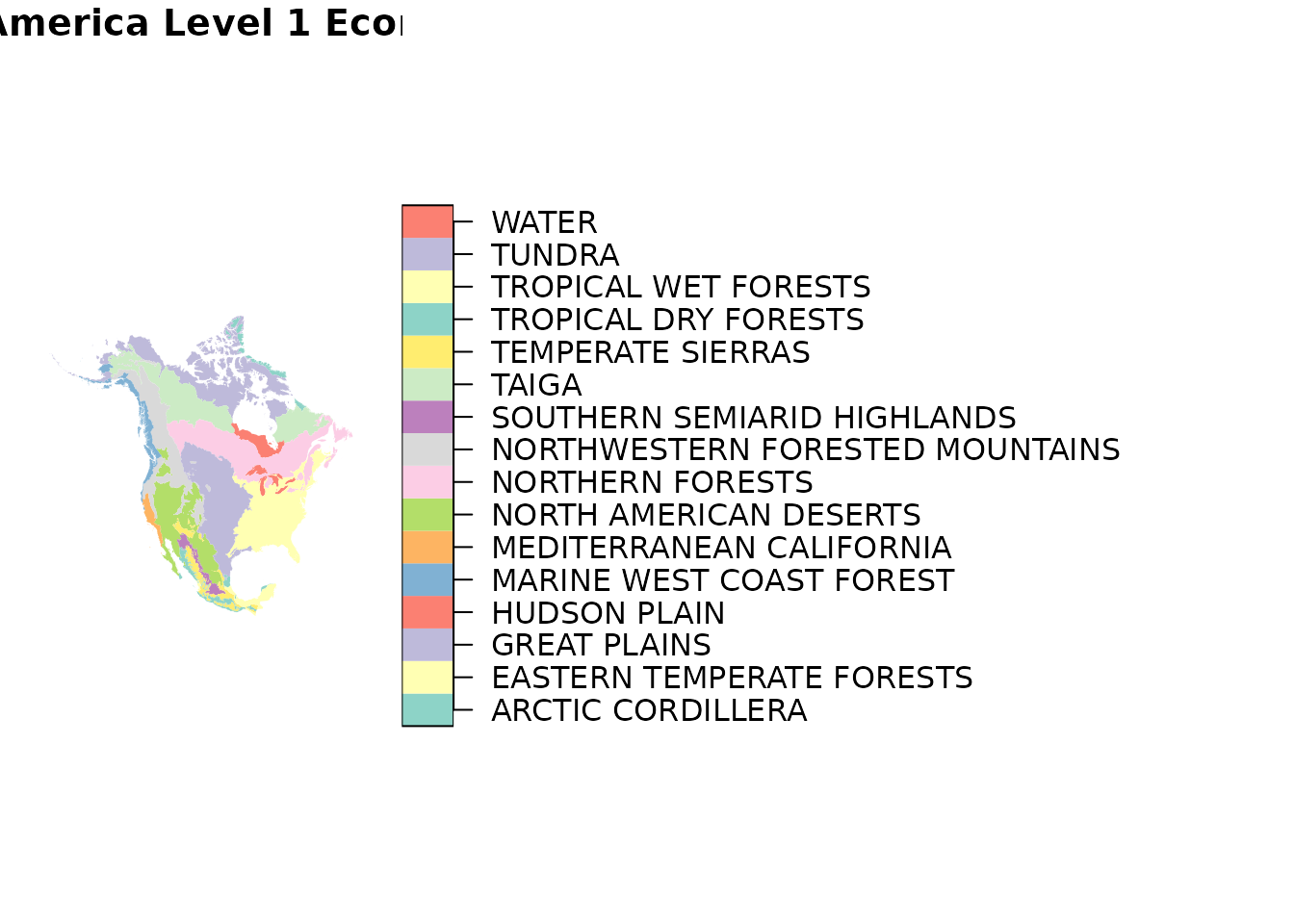
The same data rendered with ggplot2 via
geom_sf():
ggplot(na_l1) +
  geom_sf(aes(fill = NA_L1NAME), color = NA) +
  guides(fill = "none") +
  labs(title = "North America Level 1 Ecoregions") +
  theme_minimal()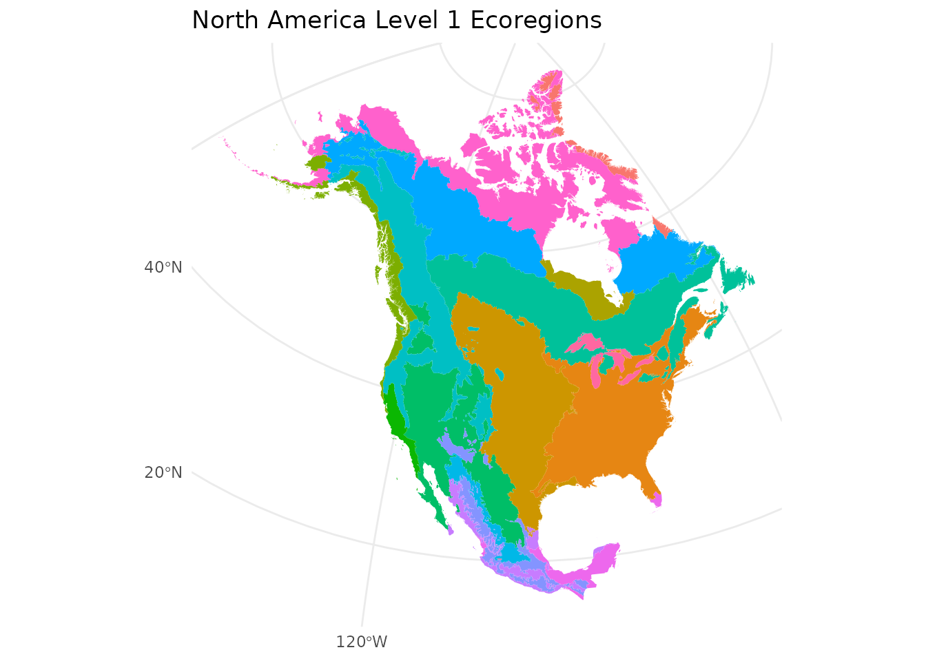
MTBS fire perimeters
All fires
With output = "sf", read_mtbs() returns an
sf object containing every fire perimeter
in the MTBS composite dataset — all years, all states.
fires <- read_mtbs(output = "sf")
fires
#> Simple feature collection with 31,386 features and 22 fields
#> Geometry type: MULTIPOLYGON
#> Dimension:     XY
#> Bounding box:  xmin: -178.3 ymin: 17.9 xmax: -65.3 ymax: 71.4
#> CRS:           NAD83 / Conus Albers (EPSG:5070)
Plot the burn area acreage to get a quick sense of the data:
plot(fires["BurnBndAc"], main = "MTBS Fire Perimeters — All Years")Filtering by year
Year range
Use R’s : operator to keep all fires within a contiguous
span of years:
Quickly visualise where the major fires of the last decade fell:
library(sf)

plot(st_geometry(fires_recent), col = "#E25822AA", border = NA,
main = "MTBS Fire Perimeters 2018–2023")Output formats
terra::SpatVector
Set output = "vect" (or "terra") to receive
a terra::SpatVector instead of an sf object —
handy when the rest of your workflow uses terra:
Attribute table only
Set geometry = FALSE to drop geometry and get a plain
data.frame. Useful when you only need the metadata (fire
name, year, acreage, etc.):
tbl <- read_mtbs(geometry = FALSE)
head(tbl[, c("Incid_Name", "Ig_Date", "BurnBndAc", "Incid_Type")])
#>     Incid_Name   Ig_Date BurnBndAc Incid_Type
#> 1  LOWDEN FIRE 1984-07-01   4537.35   Wildfire
#> 2  EUREKA FIRE 1984-08-15  11202.06   Wildfire
#> ...
Caching downloads
The MTBS ZIP archive is ~360 MB. Download it once with
get_mtbs(), then read from disk with
read_mtbs() on every subsequent call.
Default cache directory
Pass cache = TRUE to read_mtbs() to look
for the ZIP in tools::R_user_dir("fireR", "cache") — a
platform-appropriate user directory that persists between R
sessions:
# Download once to the user cache directory
get_mtbs(directory = tools::R_user_dir("fireR", "cache"))

# Read from cache on every subsequent call
fires <- read_mtbs(cache = TRUE)
Custom cache directory
Supply a directory path to both functions to control where the file is stored:
Force a fresh download
If the USGS releases an updated dataset, use
overwrite = TRUE on get_mtbs() to bypass the
cache and re-download:
get_mtbs(directory = tools::R_user_dir("fireR", "cache"), overwrite = TRUE)
fires <- read_mtbs(cache = TRUE)
Quiet mode
Progress messages are printed by default. Suppress them with
verbose = FALSE:
fires <- read_mtbs(years = 2022, verbose = FALSE)SE FireMap
get_sefire() downloads four SE FireMap data products via
the dataset argument: annual Burn Severity mosaics
(year-based, the default) and three single-file products covering
1994–2024 — Fire History, Burned Area Polygons, and Burned Area
Rasters.
Burn Severity mosaics
dataset = "Burn Severity" (the default) downloads one
Annual Burn Severity Mosaic ZIP per year for the southeastern United
States (2000–2022). Pass a single year, a range, or a vector of specific
years:
# Single year
zip_path <- get_sefire(years = 2020)
# Contiguous range
zip_paths <- get_sefire(years = 2015:2020, directory = "data/sefire")
# Specific years only
zip_paths <- get_sefire(years = c(2000, 2010, 2020))
Single-file datasets (1994–2024)
The remaining three datasets are each a single geodatabase ZIP
covering 1994–2024. The years argument does not apply to
them:
# Fire History
zip_path <- get_sefire(dataset = "Fire History", directory = "data/sefire")
# Burned Area Polygons
zip_path <- get_sefire(dataset = "Burned Area Polygons", directory = "data/sefire")
# Burned Area Rasters
zip_path <- get_sefire(dataset = "Burned Area Rasters", directory = "data/sefire")
NIFC wildfire perimeters
get_nifc() downloads the NIFC wildfire perimeters ZIP;
read_nifc() reads and filters it, with optional year
filtering via the FireYear column:
# Download once
get_nifc(directory = "data/nifc")

# Read all perimeters, or filter by year
perims      <- read_nifc(cache = "data/nifc", output = "sf")
perims_2021 <- read_nifc(cache = "data/nifc", years = 2021)
USFS Fire Occurrence Database (FPA-FOD)
get_fod() downloads the FPA-FOD GeoPackage ZIP;
read_fod() reads and filters it. The dataset covers
1992–2020 (FIRE_YEAR column):
Wildland-Urban Interface (WUI)
get_wui() downloads the USFS Wildland-Urban Interface
dataset, which delineates areas where structures meet or intermingle
with undeveloped wildland vegetation. The ZIP is very large
(~4.65 GB), and the function warns about this before
downloading. The recommended pattern is to run the download in a
background R session with callr::r_bg() so your console
stays free:
# Recommended: run in a background session (4.65 GB download)
bg <- callr::r_bg(function() fireR::get_wui(directory = "data/wui"))
bg$wait()

# Or download directly in the current session
zip_path <- get_wui(directory = "data/wui")
Ecoregion boundaries
North America (CEC Levels 1–3)
The Commission for Environmental Cooperation (CEC) ecoregion framework divides North America into hierarchical ecological units.
# Level 1 — broadest continental divisions
na_l1 <- get_nal1eco()

# Level 2 — finer continental subdivisions
na_l2 <- get_nal2eco()

# Level 3 — finest continental scale (= US EPA Level III)
na_l3 <- get_nal3eco()

plot(na_l1["NA_L1NAME"], main = "North America Level 1 Ecoregions")
US EPA (Levels 3–4)
US EPA ecoregions are available at Levels 3 and 4, with an option to include state boundaries in the polygons.
# Level 3 — without state boundaries (default)
us_l3 <- get_usl3eco()

# Level 3 — with state boundaries dissolved in
us_l3_states <- get_usl3eco(state = TRUE)

# Level 4 — finest US subdivisions
us_l4 <- get_usl4eco()
us_l4_states <- get_usl4eco(state = TRUE)
All ecoregion functions accept output = "vect" for a
terra::SpatVector and a cache argument to
persist downloads across sessions:
us_l3 <- get_usl3eco(output = "vect", cache = TRUE)Working with the data
Once you have an sf object, the full sf
and dplyr ecosystem is available to you.
Key MTBS columns
| Column | Description |
|---|---|
Incid_Name |
Name of the fire event |
Ig_Date |
Ignition date (YYYY-MM-DD) |
BurnBndAc |
Burned area in acres |
Incid_Type |
Incident type (Wildfire, Prescribed Fire, etc.) |
irwinID |
Unique IRWIN identifier |
geometry |
Fire perimeter polygon(s) |
Example: area burned and fires per year
fires_all |>
  st_drop_geometry() |>
  mutate(year = as.integer(substr(Ig_Date, 1, 4))) |>
  group_by(year) |>
  summarize(area_burned = sum(BurnBndAc)) |>
  ggplot(aes(year, area_burned)) +
  geom_col(fill = "#8B1A1A") +
  labs(title = "Area Burned by Year",
       x = "Year",
       y = "Area Burned (Acres)") +
  theme_classic()
fires_all |>
  st_drop_geometry() |>
  mutate(year = as.integer(substr(Ig_Date, 1, 4))) |>
  count(year) |>
  ggplot(aes(year, n)) +
  geom_col(fill = "#8B1A1A") +
  labs(title = "Number of Fires by Year",
       x = "Year",
       y = "Number of Fires") +
  theme_classic()
About MTBS
The Monitoring Trends in Burn Severity programme is a joint USGS / USFS initiative that maps the location, extent, and burn severity of all large wildfires (>1 000 acres in the western US; >500 acres in the eastern US) across the conterminous USA, Alaska, Hawaii, and Puerto Rico from 1984 to the present.
More information: https://www.mtbs.gov/